Colorado School of Mines Research

Synthesis and Propulsion of Magnetic Microrobots

1 Background

Asymmetric, magnetic dimers show good potential for being used as the building blocks for micro-robots. The unbalanced electrohydrodynamic (EHD) flow surrounding these dimers causes linear and circular motion. By tuning the zeta potential of the dimers, as well as the magnitude and frequency of both the electric and magnetic fields that create the EHD flow, we can control the dimers such that their behavior matches that of a micro-car, which is necessary for cargo delivery and other applications.

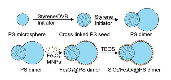
Figure 1: Synthesis of magnetic dimers used for robots.

2 Research Goals

Synthesize stable, functional magnetic dimer particles
Determine the relationship between the applied magnetic frequency and the rotational frequency of the dimers
Accurately control the motion of the magnetic particles using computational trajectories
Test different kinds of magnetic-electric field combinations in order to manufacture unique motion

3 Apparatus

Substrate with dimers

AC electric field

X-Y Helmholtz coil

Plastic stand

Figure 2: Apparatus used for experimentation

4 Results

Determining critical rotation frequency for magnetic fields:

Figure 3: a) Rotational frequency of dimers versus the frequency and strength of the applied magnetic field. Note the different in theoretical versus experimental rotation speed at high magnetic frequencies, caused by the phase lag between the induced dipoles. b) The critical frequency versus the strength of magnetic field, displaying a linear relationship.

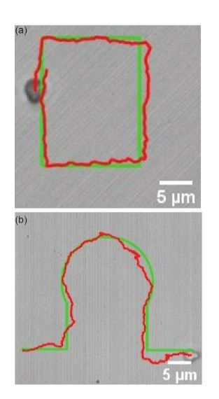
Trajectory-tracing using dynamic electric/magnetic field:

Figure 4: a) The rectangular-shaped trajectory of a dimer drawn by combined fields (8 Vpp, 400 Hz electric field and 1.1 mT DC magnetic field). b) The omega-shaped trajectory of a dimer drawn by combined fields (12 Vpp, 1,000 Hz electric field and 1.1 mT DC magnetic field). The red lines are the particle's actual trajectory, and the green line is the trajectory intended by the programmed magnetic and electric field.

5 Conclusions and Future Work

Our method for synthesizing magnetic dimers return particles that repeatedly respond to magnetic and electric field manipulation. Our experimental results for the critical rotational frequency of the dimers matched the expected models we ran prior to testing. We have demonstrated a method for controlling the motion of anisotropic particles in a precise and accurate manner. Using these methods, the dimers could be used for colloidal assembly, micromachines, and cargo delivery.

First, we want to synthesize magnetic dimers with fewer impurities in a repeatable process. We want to continue testing different electric/magnetic field combinations in order to find unique motion. Using the methods from this project, we look to apply them to creating crystalline structure inside of wedge device using PS particles and Dynabeads

References

[1] Kim, H.; Furst, E. M. Magnetic Properties, Responsiveness, and Stability of Paramagnetic Dumbbell and Ellipsoid Colloids. Journal of Colloid and Interface Science 2020, 566, 419–426.
[2] Ma, F.; Wang, S.; Wu, D. T.; Wu, N. Electric-Field-Induced Assembly and Propulsion of Chiral Colloidal Clusters. Proceedings of the National Academy of Sciences of the United States of America 2015, 112, 6307–6312.
[3] Ma, F.; Yang, X.; Zhao, H.; Wu, N. Inducing Propulsion of Colloidal Dimers by Breaking the Symmetry in Electrohydrodynamic Flow. Physical Review Letters 2015, 115, 208302.

Ultra High Energy Cosmic Ray Detector Simulation Analysis

1 Introduction

The two major ultra-high energy cosmic ray (UHECR) observatories, the Pierre Auger Observatory (PAO) in Malargue, Argentina and the Telescope Array (TA) located in Delta, Utah, require a cross-calibration to determine the cause of inconsistency between their observations. The detectors are measuring cosmic ray events using two different types of detection methods, meaning there are two possible reasons for incongruity: first, the two detectors are in different hemispheres, and are therefore looking at different parts of the universe, meaning both observations could be correct, and the readings for different parts of the universe
don’t align. Second, the two detectors use different kinds of detection methods [PAO uses a Water Cherenkov Detector (WCD) Surface Detector (SD) while TA uses a scintillation detector (SD)] and because of the experimental difference and implicit bias, the data measured doesn’t match.
To determine if this difference is the reason for the inconsistency and perform the cross-calibration between the two detectors, the research team is building a WCD micro-array (single hexagon stations, SHS) inside the TA array (full array stations, FAS), which is known as Auger@TA. However, the WCD detectors located within the micro-array will only have one single photomultiplier tube (PMT) to measure the radiation emitted when a cosmic ray event occurs, unlike the PAO detectors which use three PMTs, which reduces signal-to-noise ratio. To ensure that a single hexagon micro-array can recover reconstructed values like a full array, simulations should be run that identify their explicit differences.

1.1 Auger vs. TA Detectors

Auger and TA use different experimental methods for detecting ultra-high energy cosmic rays (UHECR). Auger uses a water Cherenkov surface detector, which is a tank of pure water monitored by three PMTs. Charged particles from high energy cosmic ray showers enter the tank creating Cherenkov. Cherenkov light is produced by relativistic charged particles entering the water, and the light is measured by the PMTs. The measurement is used to reconstruct the number of particles hitting the SD. It can then be used with the signal from the stations to reconstruct the properties of the primary signal produced by the original cosmic ray event. The tank is sealed, has an inner reflective surface, and is coated with carbon black to guarantee light tightness. By creating an array of these detectors spaced out over large distances, the direction and energy of the incoming cosmic ray can be measured. The SD stations at Auger are independent, powered by solar panels connected to rechargeable batteries and controlled by telecommunications. The water inside the tank is ultra-pure to ensure that bacteria doesn’t grow inside the tanks over time and distort the event measurements. Figure 1 shows a full schematic and image of one of the detectors in Argentina. Auger has 1660 of these detector stations mapped throughout the 10,370 km^2 of land.

TA uses a scintillation surface detector, a box made of two plastic scintillator layers, with a stainless-steel plate inserted in between. The cosmic ray first hits the plastic scintillator,where the high energy particle is absorbed and converted into photons. These photons are counted by a PMT and the data is stored for reconstruction. The device uses two sets of scintillators and PMTs, separated by stainless-steel, as a means for cutting down on error. Like the Auger Observatory, TA uses an array of these surface detectors to construct information about the direction the cosmic ray came from, as well as its energy. The TA surface detectors use solar panels for power and telecommunication for control. TA has 507 of these detector stations mapped throughout the 780 km^2 of land. For increased accuracy, both facilities use a complementary method for measuring cosmic rays: fluorescent telescopes. When cosmic rays enter the atmosphere, they produce nitrogen fluorescence that is detectable by fluorescent telescopes, or fluorescent detectors (FD). These measurements are generally made at times when the sky is dark and clear, or else the fluorescence created isn’t bright enough. The FD measurements are primarily used for calculating the total energy of the shower, as the FDs can measure the complete path that the particle takes before reaching the ground and account for energy loss prior to hitting the surface detector. Auger utilizes four of these FDs while TA utilizes three, due to the smaller area of coverage.

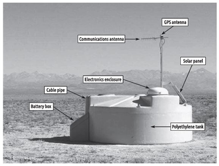
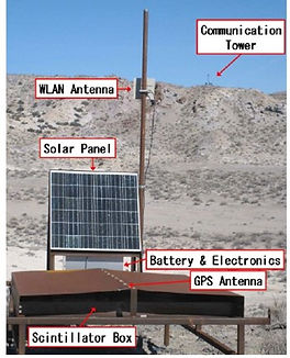
Figure 1: Schematic of (left) the water Cherenkov surface detector located at Auger and (right) the scintillation surface detector located at TA.

1.2 Phase 1 Results

The primary goals of Phase 1 of Auger@TA were integrating two WCD stations into the TA array in Utah, and then comparing the signal responses between those two WCD stations and the TA station. Unit conversion was required prior to signal comparison, since the Auger SD and TA SD stations measured spectra differently. Using local triggers, the research team found a solid correlation found between the two WCD detectors (labeled Auger North and Auger South), as can be seen by the plot in Figure 2. Grey dots represent events that triggered both the Auger North and Auger South detectors, and black dots represent events
that triggered the TA stations. A perfect result would be a slope of 1, and the experiment returned a slope of 1.1 ± 0.1, indicating that the calibration between the two Auger stations was accurate. Along with this, we can see that the black dots, indicating TA triggers, are also approximately in line with the measurements made by the Auger stations. Overall, Phase 1 confirmed the team’s ability to construct and deploy WCD detectors in Utah and cross check the local scintillation detectors. This also provided hints towards answering the questions on the disagreement between Auger and TA, but more data was needed. This motivated Phase II.

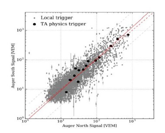
Figure 2: Auger South vs. Auger North WCD. Grey dots indicate coincident measurements (slope = 1.1±0.1) while black dots correspond to showers that also trigger the Telescope Array (slope = 1.01 ± 0.02)

1.3 Phase 2 Results

Phase 2 involves expanding this experiment from just two WCD detectors to an array of stations, like the array in Argentina, to perform a cross-calibration test at a more accurate scale. As part of Phase 2, I ran simulations that compare the results on a single PMT detector vs. a triple PMT detector. Those simulations will measure variables like the spectrum, efficiency of cosmic ray measurement, and mass composition, all in hopes
to cross-calibrate these two experimental methods more accurately. These simulations will be run on software that will output root files that will then be converted to Python for data analysis. The analysis I create will contribute directly to determining whether the data from the micro-array configuration can reconstruct values similar to the full array under specific conditions.

2 Procedures

The main task within this project was to ensure that a single hexagon micro-array can recover reconstructed values like a full array. The answer to this question is nontrivial, as an increased number of PMTs within a detector reduces the signal-to-noise ratio, making for more accurate measurements. By using simulations for both the micro-array configuration and the full array configuration, and by replicating many cosmic ray showers with varying energies and other shower variables, we gathered data that tells us whether we can develop a conclusion. The steps for programming these simulations and gathering the data are as follows:

2.1 Simulation Specifications

CORSIKA (COsmic Ray SImulations for KAscade) is used to simulate the particle cascade which results from a UHECR primary striking the atmosphere. For this work, simulated protons are in an energy range of 1 - 10 EeV with zenith angles between 0 and 65°. A random location (in a 6 by 6 km square) and azimuth angle is chosen with respect to the observatory layout wanted (micro-array or full array) and the CORSIKA shower is placed in the simulated array. Random atmospheric muons are randomly injected into the array according to their expected natural rate. The particle density, timing and average trajectory at ground (as a function of distance from the core and azimuthal angle from the core) is read in by a software called Offline to form the CORSIKA shower footprint to carry out the simulation of detector responses. At each station location in the detector simulation the particle density, timing and trajectory footprint is sampled to generate a list of particles with the timing, energy and trajectory that would be seen from the CORSIKA shower at that station’s particular location in the simulation. Using Geant4, each particle is injected into the station. The Cherenkov emission from each of these particles in the station’s water is simulated. Each Cherenkov photon is tracked as it bounces around the inside of the tank until it either strikes a PMT or is attenuated/absorbed by either the water or the liner surface. Each PMT hit is converted to a simulated electronic pulse which is carried through a simulation of the DAQ electronics. All the PMT pulses are combined to make the station’s signal response to the injected event and a simulation of the station’s trigger process is carried out. All the stations in the event’s triggers are combined and high-level physics triggers are simulated. If an event triggers at least 3 stations with sufficient signal in each station, and the timing/footprint of the station triggers matches what would be expected for a real cosmic ray event, then the event is considered to have ’triggered’. The event is then reconstructed with the goal of extracting the properties of the particle.

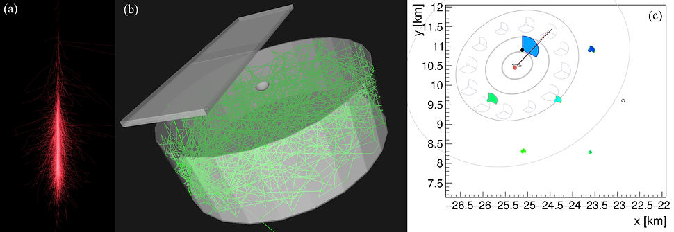
Figure 3: Images of the simulation software. (a) is an example of a CORSIKA shower. (b) is the trajectory of a photon bouncing around inside of a station. (c) is an example of what a triggered event looks like.

2.2 Simulating Cosmic Ray Showers

The cosmic ray shower simulations varied in energy, zenith and azimuth, and shower core location to get a complete representation of the behavior of both array configurations. The energy values varied from around 1018 to 1019 eV, as these are the threshold values that the PMTs are set to trigger at. Zenith angles of the cosmic showers varied from 0◦ to 65◦ [flat with respect to cos(θ)] and azimuth angles varied from 0◦ to 360◦, creating the entire spectrum of possible entrance angles. Shower core locations, or the location in the sky where the cosmic ray enters the atmosphere and becomes a large shower of particles, varied in a
4 km x 4 km square that centers on the center hexagon station. The cosmic rays were simulated hitting the array in each environment, and the data was compiled into a single file output at the end of each simulation. With both files from both simulations representing the two different environments being measured, the data was exported and analyzed further.

2.3 Analyzing the Data

The file outputs from the simulations contain a variety of quantities to be analyzed, including the thrown vs. reconstructed energies, azimuths, zeniths, and shower core axes, the number of stations that triggered for each event, the type of trigger that occurred, and other values. The filetype output by the simulation is a root file, a data structure that is unusable by the script created without some configuration and conversion prior to plots being made. Using an algorithm, a list of cosmic events with both SHS and FAS simulation reconstructions is output, one that is ready for further analysis.

3 Procedures

Shower core locations vary within a 4 km square, with the micro-array hexagon positioned at the center of the square within the full array. To reconstruct an event, three stations within the array are required to trigger, or recognize that a cosmic event has occurred due to the Cherenkov radiation created. If a cosmic event occurs further away from a station, less radiation is detected, meaning it is less likely that the station will reach the threshold required to trigger. Reconstruction is necessary to approximate the energy, zenith, azimuth,
etc. of the cosmic event, therefore determining the positions of cosmic events that result in reconstruction in either configuration (full array or micro-array) is important. Figure 4 visualizes locations of the shower cores and whether the event was reconstructed by the array. From Figure 4, we can see that for the micro-array to trigger, the location of the shower core essentially needs to be contained within the hexagon, whereas the full array can reconstruct almost every event thrown in the 4 km square. Therefore, to get the best reconstruction
comparison, we limited our data set to only events that landed inside the hexagon.

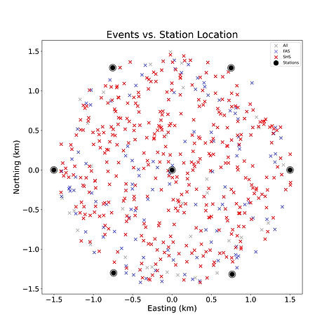
Figure 4: (left) Shower core locations reconstructed by varying arrays (micro-array stations shown only). (right) Shower Core Locations of events that landed inside the hexagon, reconstructed by varying arrays (micro-array stations shown only)

To quantify exactly how far an event on average can be away from the micro-array, and still be reconstructed, our research group developed a metric, described by Equation 1.

(1)

where M is the metric, N_μa is the number of stations in the micro-array, r_i is the location of a station, and r_core is the location of the shower core. The metric is the average distance from the core to all of the stations in the micro-array. By looking at the metric of each of the events reconstructed by the micro-array compared to that of the full array, we gathered more information about the optimal location for shower cores.

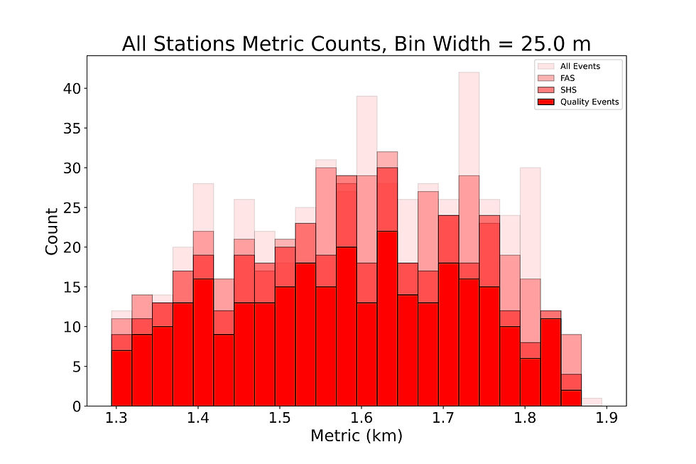
all_stations_reconstructed_metric_hist_0.025.jpg

Figure 5: Metric vs. Array type. Parameters for labeling an event as quality are as follows: ∆E/E ≤ 0.2, ∆θ ≤ 2◦, and ∆φsinθ ≤ 3◦.

∆ references the difference between a thrown and reconstructed value, therefore a lower ∆ value means a more accurate reconstruction. As we can see from Figure 5, the Single Hexagon is only able to reconstruct events that have a metric of less than about 2.5 km, with some exceptions. The full array is able to reconstruct all events, going up to greater than 3.5 km. Quality cuts are taken from the single hexagon distribution, and must have reconstructed values that follow the conditions described in the caption of Figure 7. Both the quality distribution and the single hexagon distribution follow a positive-skew distribution, while the full array and all events distribution seem to follow a somewhat bimodal distribution. The reasoning for this may have to do with the geometry of a hexagon. Along with comparing the locations where each array triggers, it is also essential to compare the actual values reconstructed. The first value to examine is the reconstructed log energy. Each event has an energy value thrown in the simulation, known as the Monte Carlo (MC) energy. The simulation then attempts to reconstruct that energy based on the location of the event. The difference in reconstruction energy is expected to vary, as the full array stations have three PMTs and the single hexagon stations have one PMT.

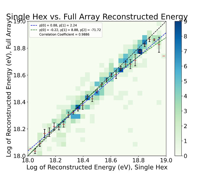
Figure 6: Heat map of reconstructed log energy values. The mean and standard deviation of each vertical distribution is overlaid on the 2D histogram. The correlation coefficient is calculated using Pearson’s r. The black dotted line represents a 1:1 fit between the single hexagon and full array reconstructions. The legend in the top left gives the parameter values of the first-order and second-order polynomial fits

Figure 6 displays the fact that there is some correlation between the reconstruction of energy in the single hexagon configuration and the reconstruction of energy in the full array configuration, but the ratio of reconstructions is not 1:1. Another key feature to examine is the trigger rates of both arrays as a function of thrown energy and azimuth. The trigger rate is defined in the following way:

(2)

Using this equation, we can bin certain variables, like energy and azimuth, and find the number of events that were triggered in that bin vs. the number of events that were thrown in that bin, with both array types. This gives us a trigger rate as a function of the value of the thrown variable.

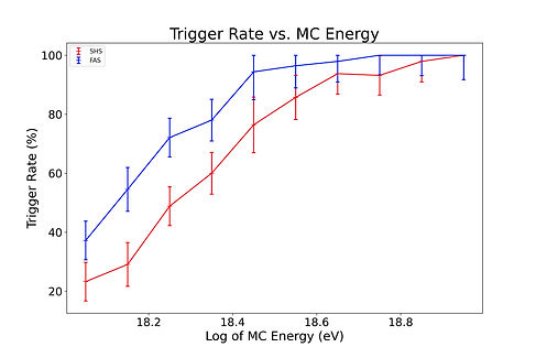
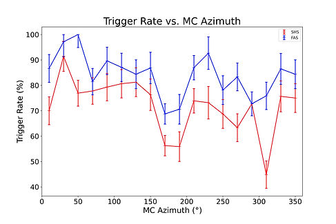
Figure 7: (left) Trigger rate as a function of MC Energy, for both FAS and SHS. Bin width is 0.1 Log eV. (right) Trigger rate as a function of MC Azimuth, for both FAS and SHS. Bin width is 10◦.

The left subfigure of Figure 7 implies that the trigger rate gets much better for both the micro-array and the full
array configurations as the energy thrown increases. This makes sense logically, as an event with a larger energy will create more radiation in a detector, making it more likely to trigger. The right subfigure of Figure 7 shows that the relationship between trigger rate and MC azimuth is nearly flat for both configurations.
Most of the plots made in this project have been replicated in other papers related to this work. However, the trigger rate plots are new pieces of information, and can provide even more information about the number of events that will be triggered in a year. By integrating over the cosmic flux, and multiplying by the trigger rate, as well as a few conversion
factors, the number of events that will be triggered on either the micro-array or full array configuration every year can be calculated.

4 Conclusions

The main argument to be made from the data collected is whether a micro-array with stations containing single PMT detectors can reconstruct UHECR values such as energy, zenith, azimuth, and trigger rate at the same level as triple PMT detectors in a full array. Of the energy range that was investigated (1-10 EeV), for the micro-array configuration to accurately reconstruct UHECR events, those events must be located within the hexagon. Events outside the hexagon cannot be reconstructed by the micro-array. When the events follow such conditions, Figure 6 shows a 0.99 correlation coefficient between the reconstructed energies.

Additionally, referencing Figure 5, we know event landing inside of the micro-array corresponds to a metric value between 1.3 and 1.9 km, given the 1.5 km separation. Referencing Figure 7, we can confirm that the trigger efficiency gets higher as a function of MC energy for the micro-array configuration, but stays flat for the full array configuration, and that the trigger efficiency stays mostly flat as a function of MC azimuth for both the micro-array and full array configurations. We have also calculated an approximate value for the number of events per year that should be expected to be detected by the SHS, confirming that it is near the experimental value.

Code

All code can be found at https://github.com/bhanson10/Auger-TA.

References

[1] F. Sarazin, C. Covault, T. Fujii, R. Halliday, J. Johnsen, R. Lorek, T. Nonaka, S. Quinn, H. Sagawa, T. Sako, R. Sato, D. Schmidt, R. Takeishi, and the Telescope Array Collaboration, EPJ Web of Conferences 210, 05002 (2019).
[2] C. Covault, T. Fujii, R. Halliday, J. Johnsen, R. Lorek, T. Nonaka, S. Quinn, H. Sagawa, T. Sako, F. Sarazin, R. Sato, D. Schmidt, and R. Takeishi, and the Telescope Array Collaboration, EPJ Web of Conferences 210, 05004 (2019).230
[3] Pierre Auger Collaboration, NIM A798, 172 (2015).
[4] Telescope Array Collaboration, NIM A689, 87 (2012).
[5] D.Ivanov. Auger and TA WG on spectrum. ICRC 2017, PoS 498.
[6] Karlsruhe Institute of Technology. CORSIKA – an Air Shower Simulation Program. (2021).235
[7] A. Aab et al. [Pierre Auger], Phys. Rev. D 102 (2020) no.6, 062005 doi:10.1103/PhysRevD.102.062005 [arXiv:2008.06486 [astro-ph.HE]].